
The role of a Machine Learning Engineer (MLE) has rapidly bifurcated from academic data science. While traditional data science interviews focus primarily on exploratory data analysis, hypothesis testing, and statistical significance, modern MLE interview loops rigorously probe a candidate’s ability to operationalize algorithms in high-throughput, low-latency production environments. Interviewers want to know: Can you architect distributed training pipelines? How do you prevent catastrophic forgetting? What statistical tests do you execute when production models suffer from concept drift?
Failing an MLE interview rarely happens because a candidate forgot the definition of a random forest. Failures occur when candidates treat machine learning like a static Kaggle competition, ignoring data validation, pipeline latency budgets, feature stores, and automated model monitoring. In this comprehensive preparation blueprint, we analyze the Top 20 Technical Scenarios asked across tier-1 technology firms, complete with model architectural diagrams, mathematical trade-offs, and production code snippets. Evaluate your transition readiness with our Data Science Career Transition Guide, and test your Python problem-solving with our Python Interview Questions for Data Analysts.
| Interview Domain | Key Focus Areas | Sample Interview Inquiry | Evaluation Metric |
|---|---|---|---|
| ML System Design | Feature Stores, Low-Latency Serving, Caching, Shadow Deployments | “Design a real-time recommendation feed serving 50M requests/sec.” | Architectural scalability, throughput, and cold-start handling |
| Model Optimization | Quantization (INT8/FP4), Pruning, Knowledge Distillation | “How do you compress a 7B model to run on an edge mobile device?” | Inference latency vs. accuracy trade-off analysis |
| Production MLOps | Data Drift, Concept Drift, Automated Retraining, CI/CD for ML | “How do you detect when customer purchasing patterns drift post-holiday?” | Statistical testing (KS-test, PSI) and rollback triggers |
| Loss Functions & Metrics | Imbalanced Classification, Focal Loss, AUC-ROC vs. PR-AUC | “Why is Accuracy a misleading metric in fraud detection models?” | Mathematical rigor and metric alignment to business ROI |
Scenario 1: High-Throughput Production MLOps Lifecycle
The most frequent architectural round asks candidates to design an end-to-end Machine Learning pipeline that continuously trains, evaluates, deploys, and monitors models at enterprise scale.
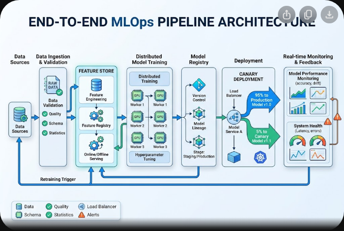
Model Architecture & Serving Strategy
Senior candidates frame their answer through the four standardized MLOps lifecycle pillars:
- Centralized Feature Store (e.g., Feast, Hopsworks): Decouples feature engineering from model training. Maintains an offline store (Snowflake, BigQuery) for historical point-in-time correct training batches, and an online store (Redis, DynamoDB) for sub-5ms low-latency feature lookups during live inference.
- Immutable Model Registry (e.g., MLflow, Weights & Biases): Tracks exact hyperparameter artifacts, training dataset Git commit hashes, environment dependencies (Docker image tags), and evaluation benchmark metrics.
- Safe Deployment Strategies (Canary & Shadow Deployments): Never route 100% of live traffic to a newly trained model immediately. Deploy a Shadow Model that receives duplicated production traffic to measure latency and error rates silently. Once validated, execute a Canary Rollout (5% $ o$ 25% $ o$ 100%) with automated rollbacks if latency spikes or user conversions degrade.
Scenario 2: Data Drift vs. Concept Drift Detection
In production, models inevitably degrade over time as real-world distributions shift. A classic interview trap asks: “Your fraud model’s F1-score dropped by 12% over the last quarter. How do you diagnose whether it is Data Drift or Concept Drift?”
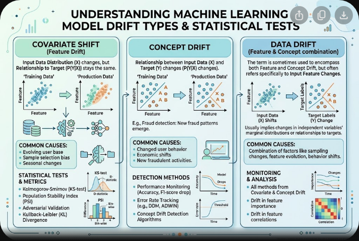
Mathematical Distinction and Statistical Testing
- Data Drift (Covariate Shift): The input feature distribution $P(X)$ changes, but the underlying conditional relationship between features and target $P(Y|X)$ remains constant. For example, users suddenly purchase via mobile devices instead of desktop, but purchasing likelihood per income bracket remains identical.
- Detection Algorithm: Run the Kolmogorov-Smirnov (KS) test for continuous features or calculate the Population Stability Index (PSI). A $ ext{PSI} > 0.25$ indicates significant distributional shift requiring automated feature recalibration.
- Concept Drift: The statistical relationship between input features and target labels $P(Y|X)$ changes fundamentally, even if input feature distributions $P(X)$ remain identical. For example, during a sudden macroeconomic inflation spike, customers with historically high credit scores suddenly begin defaulting at unprecedented rates.
- Detection Algorithm: Track sliding-window performance metrics (Precision, Recall, ROC-AUC) against verified ground truth labels using algorithms like DDM (Drift Detection Method) or ADWIN (Adaptive Windowing).
Scenario 3: Severe Class Imbalance & Loss Function Optimization
“You are training an anti-money laundering model where only 0.05% of transactions are fraudulent. Standard binary cross-entropy loss produces 99.95% accuracy by simply predicting non-fraudulent for every transaction. How do you re-architect the training objective?”
Focal Loss and Cost-Sensitive Learning
Top candidates avoid generic answers like “just use SMOTE oversampling.” Instead, they explain why modern deep learning architectures leverage Focal Loss:
# PyTorch implementation of Binary Focal Loss
import torch
import torch.nn as nn
import torch.nn.functional as F

class BinaryFocalLoss(nn.Module):
    def __init__(self, alpha=0.25, gamma=2.0):
        super(BinaryFocalLoss, self).__init__()
        self.alpha = alpha      # Balances positive vs negative importance
        self.gamma = gamma      # Focusing parameter that down-weights easy examples

    def forward(self, inputs, targets):
        BCE_loss = F.binary_cross_entropy_with_logits(inputs, targets, reduction='none')
        pt = torch.exp(-BCE_loss) # Model probability of the correct class
        F_loss = self.alpha * (1 - pt)**self.gamma * BCE_loss
        return torch.mean(F_loss)
Focal Loss applies a modulating factor $(1 – p_t)^\gamma$ to the standard cross-entropy loss. When an example is easily classified ($p_t o 1$), the factor approaches zero, drastically down-weighting the gradient contributions of millions of easy negative transactions and forcing the neural network to focus exclusively on rare, hard-to-detect fraudulent samples.
Scenario 4: Model Compression for Low-Latency Serving
“Your state-of-the-art transformer model achieves target accuracy but takes 320ms to run inference, violating the production SLA of 50ms. What engineering techniques reduce latency without sacrificing accuracy?”
The Triad of Model Compression
- Post-Training Quantization (PTQ) vs. QAT: Convert 32-bit floating-point weights (FP32) to 8-bit integers (INT8) or 4-bit representations. Quantization reduces memory bandwidth pressure by 4x and leverages hardware-accelerated integer vector instructions (e.g., INT8 Tensor Cores), typically cutting inference latency by 60–75%.
- Structured Weight Pruning: Zero out redundant neural weights or entire attention heads that contribute negligible gradient magnitudes. Structured pruning physically shrinks matrix dimensions, yielding immediate execution speedups on standard GPU hardware without requiring sparse matrix runtimes.
- Knowledge Distillation: Train a compact “Student” model to mimic the soft probability distribution (logits) generated by a massive “Teacher” ensemble. The compact student preserves over 95% of the teacher’s predictive power while running 5x to 10x faster.
To deepen your machine learning foundations, explore our guides on Statistics for Data Analysis, our Machine Learning Roadmap for Beginners, and our Data Analyst Behavioral Interview Guide.
Frequently Asked Questions (FAQ)
What is the difference between a Data Scientist and a Machine Learning Engineer?
Data Scientists primarily analyze business data, formulate statistical hypotheses, and build proof-of-concept models to inform strategic decisions. Machine Learning Engineers focus on software engineering, distributed system architecture, MLOps, and deploying scalable inference pipelines into production software.
Why is AUC-ROC often inadequate for evaluating imbalanced classification models?
The False Positive Rate (FPR) denominator in AUC-ROC includes true negatives. In heavily imbalanced problems with millions of negative samples, large absolute increases in false positives produce only tiny percentage changes in FPR, creating an artificially optimistic curve. In contrast, the Precision-Recall AUC (PR-AUC) focuses exclusively on positive predictions and true positives, exposing true model performance on rare classes.
What is the purpose of a Feature Store in enterprise ML?
Feature stores eliminate feature duplication across data science teams, guarantee consistency between offline training data and online real-time inference features, and prevent subtle “data leakage” through automated point-in-time correctness.
How do you handle cold-start problems in recommendation engines?
Cold-start issues are resolved using hybrid recommendation architectures: routing new users to popularity-based or demographic-based heuristics, utilizing content-based embeddings extracted from item metadata, and leveraging multi-armed bandit algorithms (like Thompson Sampling) to balance exploration of new items with exploitation of proven hits.
Scenario 5: Distributed Model Training and Data Parallelism
When training multi-billion parameter neural networks or processing multi-terabyte image and text datasets, single-GPU memory limits become an insurmountable bottleneck. A key interview inquiry probes how engineers scale training across distributed GPU clusters using Distributed Data Parallel (DDP) vs. Fully Sharded Data Parallel (FSDP).
DDP vs. ZeRO and FSDP
In standard PyTorch Distributed Data Parallel (DDP), the entire model architecture, optimizer states, and gradients are replicated identically across every GPU. Each device processes an independent batch slice (data parallelism) and synchronizes gradients via an AllReduce collective communication call. However, when the model itself exceeds single-GPU VRAM, DDP fails with an Out-of-Memory (OOM) exception. To solve this, FSDP (Fully Sharded Data Parallel) implements the ZeRO (Zero Redundancy Optimizer) memory-saving algorithm, sharding model weights, gradients, and optimizer states across all available cluster nodes and gathering layers dynamically on-demand during forward and backward passes. This allows engineering teams to train 10x larger architectures without requiring specialized pipeline-parallel model refactoring.